Linear Regression with Math.NET Numerics

Likely the most requested feature for Math.NET Numerics is support for some form of regression, or fitting data to a curve. I'll show in this article how you can easily compute regressions manually using Math.NET, until we support it out of the box. We already have broad interpolation support, but interpolation is about fitting some curve exactly through a given set of data points and therefore an entirely different problem.

For a regression there are usually much more data points available than curve parameters, so we want to find the parameters that produce the lowest errors on the provided data points, according to some error metric.

Least Squares Linear Regression

If the curve is linear in its parameters, then we're speaking of linear regression. The problem becomes much simpler and we can leverage the rich linear algebra toolset to find the best parameters, especially if we want to minimize the square of the errors (least squares metric).

In the general case such a curve would be in the form of a linear combination of \(N\) arbitrary but known functions \(f_i(x)\), scaled by the parameters \(p_i\). Note that none of the functions \(f_i\) depends on any of the \(p_i\) parameters.

\[y : x \mapsto p_1 f_1(x) + p_2 f_2(x) + \cdots + p_N f_N(x)\]

If we have \(M\) data points \((x_j,y_j)\), then we can write the whole problem as an overdefined system of \(M\) equations:

\[\begin{eqnarray} y_1 &=& p_1 f_1(x_1) + p_2 f_2(x_1) + \cdots + p_N f_N(x_1) \\ y_2 &=& p_1 f_1(x_2) + p_2 f_2(x_2) + \cdots + p_N f_N(x_2) \\ &\vdots& \\ y_M &=& p_1 f_1(x_M) + p_2 f_2(x_M) + \cdots + p_N f_N(x_M) \end{eqnarray}\]

Or in matrix notation:

\[\begin{eqnarray} \mathbf y &=& \mathbf X \mathbf p \\ \begin{bmatrix}y_1\\y_2\\ \vdots \\y_M\end{bmatrix} &=& \begin{bmatrix}f_1(x_1) & f_2(x_1) & \cdots & f_N(x_1)\\f_1(x_2) & f_2(x_2) & \cdots & f_N(x_2)\\ \vdots & \vdots & \ddots & \vdots\\f_1(x_M) & f_2(x_M) & \cdots & f_N(x_M)\end{bmatrix} \begin{bmatrix}p_1\\p_2\\ \vdots \\p_N\end{bmatrix} \end{eqnarray}\]

This is a standard least squares problem and can easily be solved using Math.NET Numerics's linear algebra classes and the QR decomposition. In literature you'll usually find algorithms explicitly computing some form of matrix inversion. While symbolically correct, using the QR decomposition instead is numerically more robust. This is a solved problem, after all.

1: 

var p = X.QR().Solve(y);

Some \(\mathbf{X}\) matrices of this form have well known names, for example the Vandermonde-Matrix for fitting to a polynomial.

Example: Fitting to a Line

A line can be parametrized by the height \(a\) at \(x=0\) and its slope \(b\):

\[y : x \mapsto a + b x\]

This maps to the general case with \(N=2\) parameters as follows:

\[p_1 = a, f_1 : x \mapsto 1 \\ p_2 = b, f_2 : x \mapsto x\]

And therefore the equation system

\[\begin{bmatrix}y_1\\y_2\\ \vdots \\y_M\end{bmatrix} = \begin{bmatrix}1 & x_1\\1 & x_2\\ \vdots & \vdots\\1 & x_M\end{bmatrix} \begin{bmatrix}a\\b\end{bmatrix}\]

The complete code when using Math.NET Numerics would look like this:

 1: 
 2: 
 3: 
 4: 
 5: 
 6: 
 7: 
 8: 
 9: 
10: 
11: 
12: 
13: 

// data points
var xdata = new double[] { 10, 20, 30 };
var ydata = new double[] { 15, 20, 25 };

// build matrices
var X = DenseMatrix.CreateFromColumns(
  new[] {new DenseVector(xdata.Length, 1), new DenseVector(xdata)});
var y = new DenseVector(ydata);

// solve
var p = X.QR().Solve(y);
var a = p[0];
var b = p[1];

Example: Fitting to an arbitrary linear function

The functions \(f_i(x)\) do not have to be linear in \(x\) at all to work with linear regression, as long as the resulting function \(y(x)\) remains linear in the parameters \(p_i\). In fact, we can use arbitrary functions, as long as they are defined at all our data points \(x_j\). For example, let's compute the regression to the following complicated function including the Digamma function \(\psi(x)\), sometimes also known as Psi function:

\[y : x \mapsto a \sqrt{\exp x} + b \psi(x^2)\]

The resulting equation system in Matrix form:

\[\begin{bmatrix}y_1\\y_2\\ \vdots \\y_M\end{bmatrix} = \begin{bmatrix}\sqrt{\exp{x_1}} & \psi(x_1^2)\\\sqrt{\exp{x_2}} & \psi(x_2^2)\\ \vdots & \vdots\\\sqrt{\exp{x_M}} & \psi(x_M^2)\end{bmatrix} \begin{bmatrix}a\\b\end{bmatrix}\]

The complete code with Math.NET Numerics, but this time with F#:

 1: 
 2: 
 3: 
 4: 
 5: 
 6: 
 7: 
 8: 
 9: 
10: 
11: 
12: 
13: 
14: 
15: 
16: 
17: 
18: 
19: 
20: 

// define our target functions
let f1 x = Math.Sqrt(Math.Exp(x))
let f2 x = SpecialFunctions.DiGamma(x*x)

// create data samples, with chosen parameters and with gaussian noise added
let fy (noise:IContinuousDistribution) x = 2.5*f1(x) - 4.0*f2(x) + noise.Sample()
let xdata = [ 1.0 .. 1.0 .. 10.0 ]
let ydata = xdata |> List.map (fy (Normal.WithMeanVariance(0.0,2.0)))

// build matrix form
let X =
    [|
        xdata |> List.map f1 |> vector
        xdata |> List.map f2 |> vector
    |] |> DenseMatrix.CreateFromColumns
let y = vector ydata

// solve
let p = X.QR().Solve(y)
let (a,b) = (p.[0], p.[1])

Note that we use the Math.NET Numerics F# package here (e.g. for the vector function).

Example: Fitting to a Sine

Just like the digamma function we can also target a sine curve. However, to make it more interesting, we're also looking for phase shift and frequency parameters:

\[y : x \mapsto a + b \sin(c + \omega x)\]

Unfortunately the function \(f_2 : x \mapsto \sin(c + \omega x)\) now depends on parameters \(c\) and \(\omega\) which is not allowed in linear regression. Indeed, fitting to a frequency \(\omega\) in a linear way is not trivial if possible at all, but for a fixed \(\omega\) we can leverage the following trigonometric identity:

\[\begin{eqnarray} a+b\sin(c + \omega x) &=& a+u\sin{\omega x}+v\cos{\omega x} \\ b &=& \sqrt{u^2+v^2} \\ c &=& \operatorname{atan2}(v,u) \end{eqnarray}\]

and therefore

\[\begin{bmatrix}y_1\\y_2\\ \vdots \\y_M\end{bmatrix} = \begin{bmatrix}1 & \sin \omega x_1 & \cos \omega x_1\\1 & \sin \omega x_2 & \cos \omega x_2\\ \vdots & \vdots & \vdots\\1 & \sin \omega x_M & \cos \omega x_M\end{bmatrix} \begin{bmatrix}a\\u\\v\end{bmatrix}\]

However, note that because of the non-linear transformation on the \(b\) and \(c\) parameters, the result will no longer be strictly the least square error solution. While our result would be good enough for some scenarios, we'd either need to compensate or switch to non-linear regression if we need the actual least square error parameters.

The complete code in C# with Math.NET Numerics would look like this:

 1: 
 2: 
 3: 
 4: 
 5: 
 6: 
 7: 
 8: 
 9: 
10: 
11: 
12: 
13: 
14: 
15: 
16: 
17: 
18: 
19: 

// data points: we compute y perfectly but then add strong random noise to it
var rnd = new Random(1);
var omega = 1.0d
var xdata = new double[] { -1, 0, 0.1, 0.2, 0.3, 0.4, 0.65, 1.0, 1.2, 2.1, 4.5, 5.0, 6.0 };
var ydata = xdata
  .Select(x => 5 + 2 * Math.Sin(omega*x + 0.2) + 2*(rnd.NextDouble()-0.5)).ToArray();

// build matrices
var X = Matrix.CreateFromColumns(new[] {
    new DenseVector(xdata.Length, 1),
    new DenseVector(xdata.Select(t => Math.Sin(omega*t)).ToArray()),
    new DenseVector(xdata.Select(t => Math.Cos(omega*t)).ToArray())});
var y = new DenseVector(ydata);

// solve
var p = X.QR().Solve(y);
var a = p[0];
var b = SpecialFunctions.Hypotenuse(p[1], p[2]);
var c = Math.Atan2(p[2], p[1]);

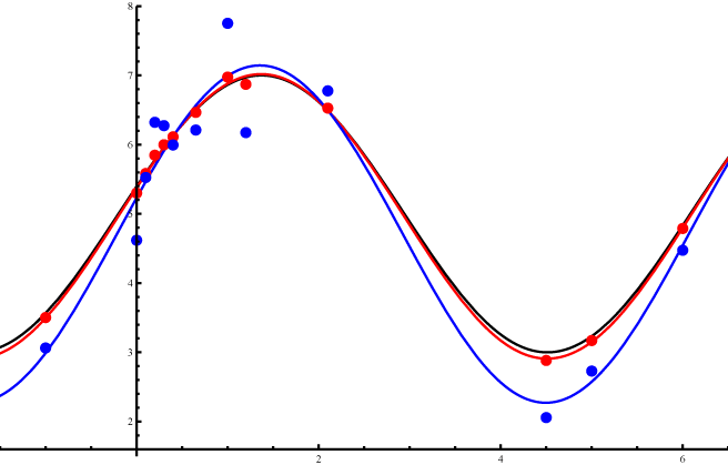
The following graph visualizes the resulting regressions. The curve we computed the \(y\) values from, before adding the strong noise, is shown in black. The red dots show the actual data points with only small noise, the blue dots the points with much stronger noise added. The red and blue curves then show the actual computed regressions for each.